Quick Start Guide - Fringe Fitting in HOPS4
This quick start guide walks through a basic fringe-fitting example using the vt9105
VGOS test dataset. By the end you will have run fourfit4 on a single
baseline, produced a fringe file, and inspected the plot and results.
Prerequisites
HOPS4 installed (with plotting enabled via gnuplot or python-matplotlib) in <hops-install> and the environment sourced:
export HOPS_INSTALL_DIR=<hops-install>
source $HOPS_INSTALL_DIR/bin/hops.bash
The
vt9105test dataset downloaded. To obtain the test data archives run:testdata_download_all.sh
This will place the data under
$HOPS_INSTALL_DIR/data/test_data/. You can then unpack it with:cd $HOPS_INSTALL_DIR/data/test_data/ tar -xzvf ./vt9105.tar.gz
Then set a shell variable for convenience:
DATADIR=$HOPS_INSTALL_DIR/data/test_data/vt9105
cd $DATADIR
Data Directory Layout
HOPS4 organizes correlation data in a two-level hierarchy (experiment, scan) which looks like:
<experiment-number>/
  <scan-directory>/
    <source>.root.json      # scan metadata
    <baseline>.cor          # correlator output (one per baseline)
    <station>.sta           # station data (one per station)
This is the same structure that was use by the Mark4 format, though the binary data format is entirely different.
As an example of the Mark4 directory structure, the vt9105 dataset contains Mark4-format data in the
experiment directory 1234 which looks like:
vt9105/
  cf_test5                 # control file for this experiment
  1234/
    105-1800/              # scan: day 105, 18:00 UTC
      0016+731.0VSI1M      # mark4 root (ovex) metadata
      G..0VSI1M            # mark4 station (G) data
      E..0VSI1M            # mark4 station (E) data
      GE..0VSI1M           # mark4 baseline (GE) visibility data
      ...
Where the directory 105-1800 is the HOPS scan directory (named by: day-of-year 105, start time 18:00 UTC).
This date-time naming convention is typical for VGOS/geodesy, but is not required by the format. The GE.. file
contains the visibility data associated with the baseline between stations G (Goddard) and E (Westford), whereas the E.. and
G.. files contain the station data (delay models, etc.).
Step 1: Convert Mark4 Data to HOPS4 Format
Since fourfit4 reads the new HOPS4 .cor/.sta file format, the first step in this example is
to use mark42hops to convert the Mark4 data in 1234/105-1800 to the HOPS4 format, writing output into 1111/105-1800b:
mkdir -p ./1111
mark42hops -i ./1234/105-1800 -o ./1111/105-1800b
mark42hops reads every baseline and station file from the Mark4 scan
directory and writes the equivalent HOPS4 .cor, .sta, and
.root.json files to the output directory. This produces:
vt9105/
  1111/
    105-1800b/                    # scan: day 105, 18:00 UTC
      0016+731.0VSI1M.root.json   # hops4 metadata
      G.Gs.0VSI1M.sta             # hops4 station (G) data
      E.Wf.0VSI1M.sta             # hops4 station (E) data
      GE.Gs-Wf.0VSI1M.cor         # mark4 baseline (GE) visibility data
      ...
Note
The experiment vt9105 also contains .difx output. If you have the DiFX difxio library available and have
enabled HOPS_USE_DIFXIO=ON, you can use difx2hops instead to produce HOPS4 data directly from the DiFX files.
This is the standard path for processing data in HOPS4 (conversion from the Mark4 format is provided for backwards compatibility).
Note
fourfit4 expects data in the HOPS4 format. However, the -K (uppercase) flag can be passed to fourfit4 to
tell it to consume mark4 formatted data directly. This is recommended only for quick one-off inspection, as it requires
a temporary data copy (in /dev/shm if available, otherwise /tmp) to do the conversion from the Mark4 to HOPS4 format. This is not as efficient as
pre-converting the data. Similarly, fourfit4 will generate output in the HOPS4 format. However, the user may
pass the -k (lowercase) flag which will cause fourfit4 to generate legacy Mark4 fringe output files
(e.g. GE.X.1.0VSI1M) instead of HOPS4 format .frng files irrespective of the input format.
Step 2: The Control File
The fourfit control file sets fringe-search parameters and per-station calibration
values. The test dataset includes a file: cf_test5 which is configured for this
experiment. Some of the key global parameters are:
sb_win -6.0 6.0          * single-band delay search window (us)
dr_win -5.e-6  5.e-6     * delay-rate search window (s/s)

pc_mode  multitone        * multi-tone phase calibration
pc_period 5               * phase-cal extraction period (s)

mbd_anchor sbd            * anchor multi-band delay to SBD solution
samplers 4 abcdefgh ijklmnop qrstuvwx yzABCDEF
                          * 4 samplers, 8 channels each (32 total)
ref_freq 6000.0           * reference frequency (MHz)
The file also contains additional conditional if station <X> blocks with per-station sampler
delays and manual phase-cal phases derived from a prior processing pass, used to align delay and phase across all four VGOS frequency bands.
Step 3: Run fourfit4
Note
fourfit4 --help will print a usage description of all of the command line arguments supported by fourfit4
Run fourfit4 to fringe-fit the GE baseline visibility data, generating a pseudo-Stokes-I polarization
(a normalized sum of XX, YY, XY, YX polarization products) fringe file:
fourfit4 -m -2 -c ./cf_test5 -b GE -P I ./1111/105-1800b/
Key options:
|
Message level -2 (debug-level output). |
|
Control file to use. |
|
Process only the GE baseline (omit to process all baselines). |
|
Polarization product: |
After running this command you will have a new .frng file in the scan directory alongside the .sta and .cor files.
ls ./1111/105-1800b/*frng*
./1111/105-1800b/GE.Gs-Wf.X.I.0VSI1M.1.frng
Step 4: Understanding the Output Filename
HOPS4 fringe files follow the naming convention:
<baseline>.<ref-code>-<rem-code>.<band>.<pol>.<root-code>.<n>.frng
For the file above:
|
Baseline: stations G (Goddard) and E (Westford). |
|
Station codes from the VEX file. |
|
Frequency band. |
|
Polarization product (pseudo-Stokes I) (could also be XX, YY, XY, YX, RR, LL, etc.). |
|
Root code: a short 6-char identifier for the scan derived from the creation time. |
|
Sequential fringe index (incremented for each additional fringe file in the scan directory). |
|
HOPS4 fringe file (binary data). |
Note
fourfit4 will not overwrite previously generated .frng files
(even if the exact same command/control parameters as used in a previous
run were passed). Instead it will generate a new .frng file with the
sequence number incremented by one. Use the -t option to run a fringe
fitting pass without writing output.
Step 5: Inspect the Result
Fringe plot. Display a fringe plot:
fplot4 ./1111/105-1800b/GE.Gs-Wf.X.I.0VSI1M.1.frng
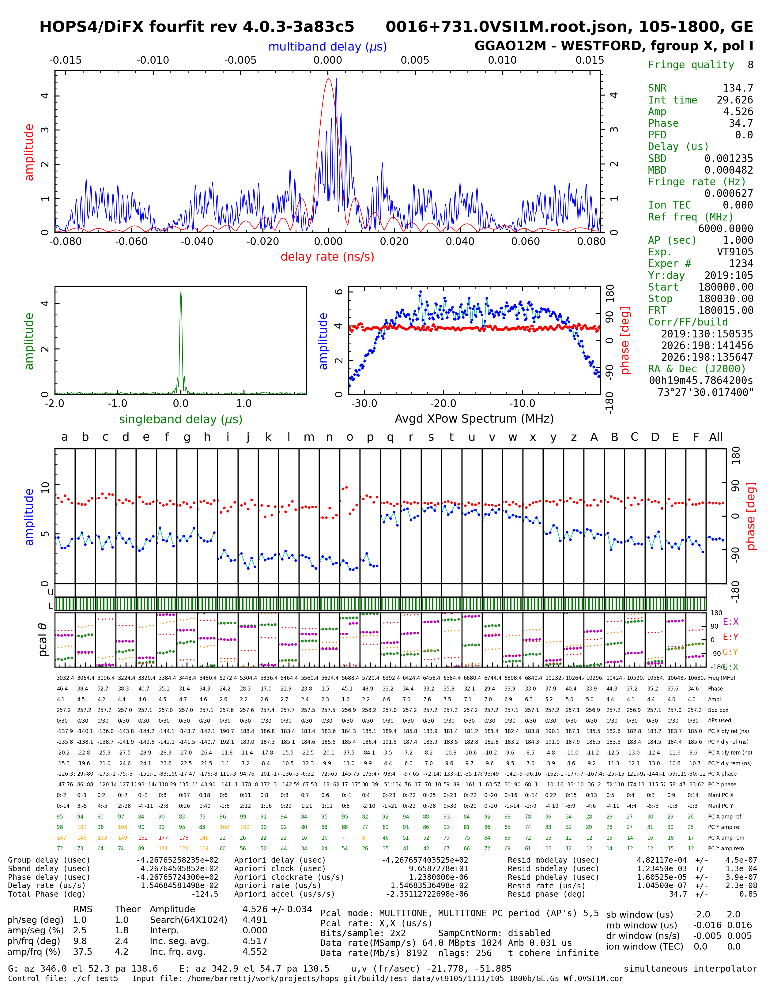
Example fringe plot generated by fplot4.
The default plotting backend for fplot4 is the gnuplot based system, which generates a fast, but static, plot. However, if you
have the python dependencies installed, you can change the plotting backend to matplotlib by using -B matplotlib.
In addition, plots can be created directly while running fourfit by passing the -p option.
JSON export. Convert the fringe file to JSON for direct data inspection:
hops2json ./1111/105-1800b/GE.Gs-Wf.X.I.0VSI1M.1.frng
This produces the file GE.Gs-Wf.X.I.0VSI1M.1.frng.json containing the
full fringe data and metadata in json format.
Note
hops2json --help describes the usage options of this conversion utility, which can also be used on .cor and .sta files.
From the JSON file you can then extract fringe data and related quantities using the command
line tool jq (See: https://jqlang.org/). For example, the following:
jq '.[].tags.plot_data | select( . != null )' ./1111/105-1800b/GE.Gs-Wf.X.I.0VSI1M.1.frng.json
will dump a json blob containing all of the plot data in the fringe file to stdout.
For more in-depth command-line exploration, use a tool like jless (From: https://jless.io/) to interactively navigate the
file structure.
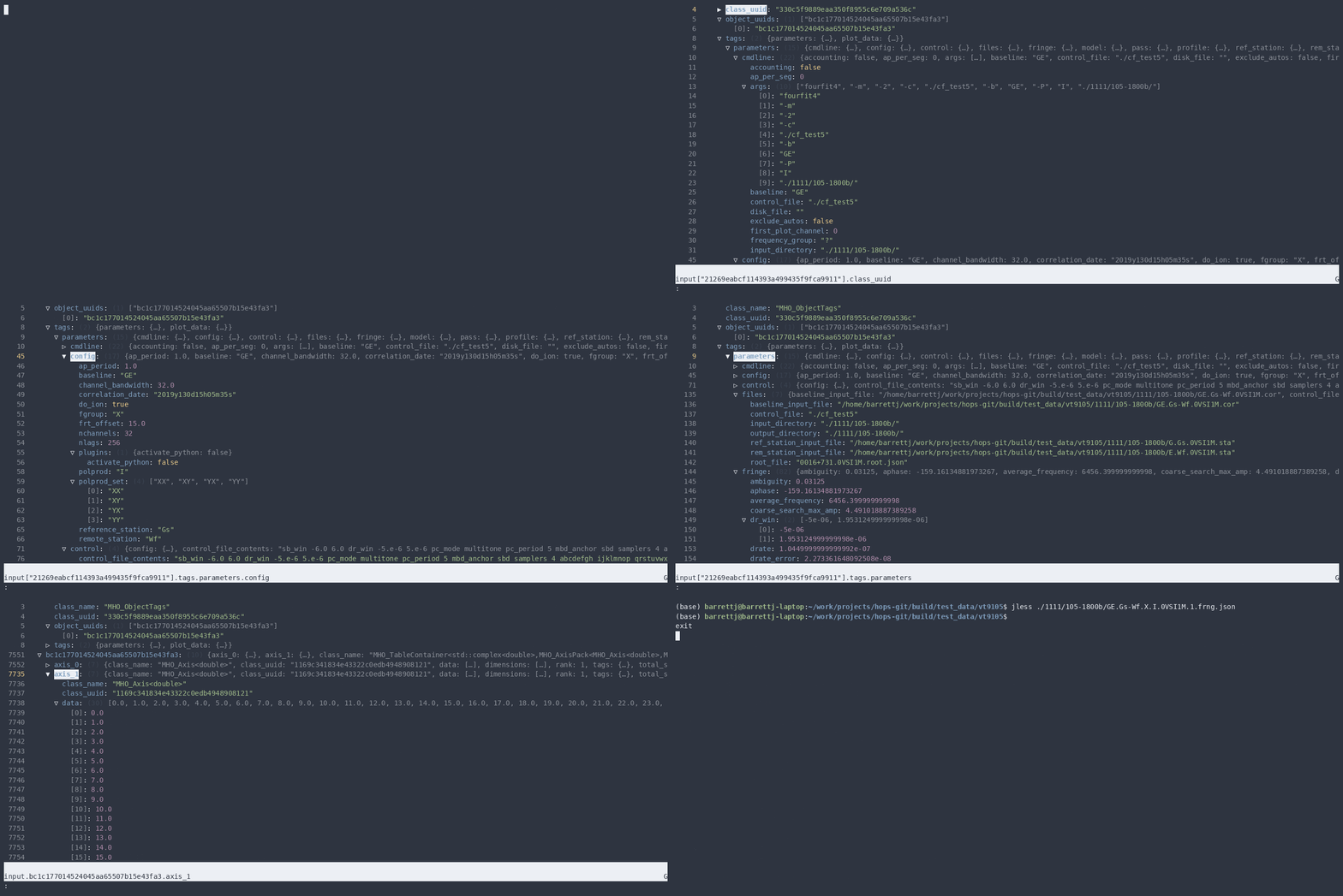
Navigating a nested HOPS4 fringe file (converted to .json) structure with jless.
For more complicated data-inspection tasks for which performance is not a concern, you can also load a .json file directly into a python dictionary via:
import json
fringe_file = "./1111/105-1800b/GE.Gs-Wf.X.I.0VSI1M.1.frng.json"

# Open and parse the JSON file
with open(fringe_file, "r") as f:
    data = json.load(f)

# 'data' is now a Python dictionary
print(data)
A-format summary. In addition, you can also generate an alist-style summary of all HOPS4 fringe files in the scan directory with:
alist4 -o ./alist.out ./1111/105-1800b/*.frng
Next Steps
Run
fourfit4with-P XXor-P YXto process a single polarization product.Run
fourfit4with-ptto generate an on-the-fly plot but without creating any fringe files.Run
fourfit4without-b GEto process all baselines in the scan in sequence.Adjust
sb_winanddr_winin the control file to change the search range.See the HOPS Python Plugin User Guide guide for writing Python plugins to customize calibration/post-processing.
See the Control File Keyword Reference for a complete list of control file keywords.